

In an era saturated with data, whether tracking personal fitness metrics like cycling distances or analyzing broad economic trends, the term “average” is ubiquitous. It serves as a single number often presumed to best represent a vast collection of information, offering a quick summary. However, beneath this seemingly simple concept lies a rich and complex landscape of statistical methods, each designed to capture a different facet of data centrality.
Indeed, relying solely on a singular interpretation of “average” can sometimes obscure more than it reveals. Just as average cycling distances might vary significantly across different age groups or training regimens, the method used to calculate that average fundamentally shapes the insights derived. To truly understand data, especially when challenged to interpret nuanced patterns, a deeper dive into the various types of averages becomes not just helpful, but essential.
This article aims to unpack the diverse world of averages, providing a clear and accessible guide to their definitions, applications, and inherent limitations. By dissecting these foundational statistical tools, we can move beyond superficial interpretations, equipping ourselves to critically analyze data, from the average miles logged by cyclists of different ages on platforms like Strava and Ride with GPS to broader statistical endeavors, ensuring our conclusions are as robust and informative as possible.
1. **Arithmetic Mean**
The arithmetic mean, often simply referred to as “the average,” stands as the most commonly understood measure of central tendency. In ordinary language, an average is indeed a single number or value that best represents a set of data. This fundamental statistic is calculated by summing all the numbers in a given list and then dividing that total by the count of numbers present in the list.
Mathematically, the arithmetic mean (denoted as x̄ or the Greek letter “μ”) is expressed by the formula: x ¯ = 1 n ∑ i = 1 n x i. For instance, if we consider a list of numbers such as 2, 3, 4, 7, and 9, their sum is 25. Dividing this sum by the count of numbers, which is 5, yields an arithmetic mean of 5. This straightforward calculation makes it a powerful and widely adopted tool for initial data summarization.
Several universal properties characterize the arithmetic mean and many other types of averages. One such property is that if all numbers in a list are identical, their average will also be equal to that number. Furthermore, the arithmetic mean exhibits monotonicity: if two lists of numbers, A and B, have the same length, and every entry in list A is at least as large as its corresponding entry in list B, then the average of list A will be at least that of list B. Another key property is linear homogeneity, meaning if all numbers in a list are multiplied by the same positive number, the average will change by that exact same factor.
However, it’s also important to acknowledge that the arithmetic mean, despite its prevalence, can be susceptible to extreme values or outliers. Its calculation considers every data point equally, meaning a few exceptionally high or low values can disproportionately influence the final average. This characteristic is precisely why understanding alternative measures of central tendency becomes critical for a comprehensive data analysis, preventing potential misinterpretations when data distributions are skewed.
In the context of optimization, the arithmetic mean can be understood as the value ‘x’ that minimizes the sum of squared differences between itself and all data points. This is represented as argmin x ∈ R ∑ i = 1 n ( x − x i ) 2. This mathematical property highlights its role in providing a central point that is, in a squared sense, closest to all the data points in the set, underlying its statistical significance.
Read more about: Seven: The Number That’s Everywhere – From Ancient Mysteries to Viral TikToks!
2. **Median*
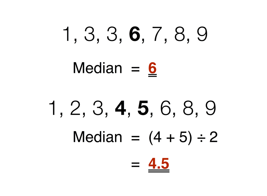
The median offers an alternative perspective on the “middle” of a dataset, distinct from the arithmetic mean. It is defined as the middle value that effectively separates the greater half from the lesser half of a data set. To determine the median, the numbers in the list must first be ranked in order of their magnitude. Once ordered, the median is the value that sits precisely in the middle.
Consider the ordered list of values {1, 2, 2, 3, 4, 7, 9}. In this set of seven numbers, 3 is the median because it is the central value. If there is an even number of numbers in the list, the median is calculated as the arithmetic mean of the two middle values. For example, in the ordered list {1, 3, 7, 13}, the two middle numbers are 3 and 7. Their arithmetic mean, (3 + 7) / 2 = 5, becomes the median.
The median is particularly valuable in situations where data might be skewed by extreme values, making it a more robust measure of central tendency compared to the arithmetic mean. For instance, the average personal income is frequently reported as the median rather than the mean. This is because the mean would be significantly inflated by the comparatively few billionaires, whereas the median more accurately represents the income level around which 50% of the population earns more and 50% earns less.
The process of finding the median involves repeatedly removing the pair consisting of the highest and lowest values from an ordered list until either one or two values remain. If a single value is left, that is the median. If two values remain, their arithmetic mean is the median. This methodical approach ensures that the median truly reflects the distributional center, unaffected by distant outliers.
From an optimization standpoint, the median minimizes the sum of absolute differences between itself and all data points. This is formalized as argmin x ∈ R ∑ i = 1 n | x − x i |. This property underscores why the median is less sensitive to outliers; it seeks to minimize linear deviations rather than squared deviations, which amplify the impact of extreme values.
Read more about: Inside the Culture Wars: 14 Celebrities Who Dared to Defy Woke Culture and Faced the Fallout

3. **Mode**
The mode provides another distinct measure of central tendency, focusing on the frequency of values within a dataset. Simply put, the mode is defined as the most frequently occurring number in a list. It identifies the value that appears with the highest frequency, offering insight into the most common observation within a data set.
For example, if we consider the list of numbers {1, 2, 2, 3, 4, 7, 9}, the number 2 appears twice, which is more often than any other number. Therefore, 2 is the mode of this dataset. Similarly, in the list {1, 2, 2, 3, 3, 3, 4}, the number 3 is the mode because it occurs three times, surpassing the frequency of other numbers.
One interesting characteristic of the mode is that a dataset can have more than one mode, or even no mode at all. It may happen that there are two or more numbers which occur equally often and more often than any other number. In such cases, there is no universally agreed-upon definition. Some authors contend that all these frequently occurring numbers are considered modes, leading to a bimodal or multimodal distribution, while others argue that if there isn’t a single most frequent value, then there is no mode.
Unlike the arithmetic mean and median, the mode can be applied to qualitative or categorical data, not just numerical data. For instance, if surveying favorite colors, the mode would simply be the color chosen by the most people. This versatility makes the mode a useful statistic for understanding common preferences or categories within various types of datasets, including those without a natural numerical order.
In terms of optimization, the mode can be seen as the value ‘x’ that maximizes the count of occurrences where ‘x’ is equal to a data point. This is expressed as argmax x ∈ R ∑ i = 1 n ( { 1 , if x = x i 0 , if x ≠ x i ). This formulation clearly highlights its role in identifying the most prevalent element within a collection of data points.
Read more about: You Won’t Believe These 10 Iconic On-Screen Couples Who Couldn’t Stand Each Other in Real Life!

4. **Mid-range**
The mid-range is a simple yet informative measure of central tendency that relies solely on the extreme values within a dataset. It is defined as the arithmetic mean of the highest and lowest values of a set. This makes its calculation straightforward and easily understood, often serving as a quick estimate for the center of a distribution.
To illustrate, consider the set of values {1, 2, 2, 3, 4, 7, 9}. The lowest value in this set is 1, and the highest value is 9. Calculating the mid-range involves adding these two extreme values and dividing by two: (1 + 9) / 2 = 5. This result provides a central point based on the span of the data, rather than the sum or order of all individual values.
Historically, the mid-range has a notable place in the development of statistical thought. It is considered a possible precursor to the arithmetic mean, with its use recorded in Arabian astronomy between the ninth and eleventh centuries. Beyond astronomy, it also found application in fields like metallurgy and navigation, where quick estimates of central values from potentially noisy measurements were valuable. This early adoption underscores its utility for practical estimation.
While easy to compute, the mid-range is highly sensitive to outliers. Because it only considers the absolute minimum and maximum values, a single unusually low or high data point can drastically alter its outcome, making it less robust than the median or even the arithmetic mean for skewed distributions. Therefore, while useful for specific contexts, its application often warrants caution and consideration of other central tendency measures.
Despite its simplicity and sensitivity to outliers, the mid-range still offers unique insights, especially when the range of data itself is a key point of interest. It efficiently captures the central point of the dataset’s overall spread. From an optimization perspective, the mid-range can be formulated as the value ‘x’ that minimizes the maximum absolute difference between ‘x’ and any data point, i.e., argmin x ∈ R max i ∈ { 1 , … , n } | x − x i |. This highlights its role in finding the center of the smallest interval containing all data points.
Read more about: Unlock a Decade of Durability: 15 Top Chef Secrets to Keeping Your Non-Stick Pans Pristine and Performing

5. **Geometric Mean**
The geometric mean is a powerful and often misunderstood average, forming one of the three classical Pythagorean means alongside the arithmetic and harmonic means. Unlike the arithmetic mean which sums values, the geometric mean is calculated by taking the nth root of the product of all the given numbers, where ‘n’ is the count of those numbers. This makes it particularly suitable for datasets involving growth rates, ratios, or values that are multiplied together.
The formula for the geometric mean is G.M. = n√(x 1 .x 2 …x n ), or more generally, ∏ i = 1 n x i n = x 1 ⋅ x 2 ⋯ x n n. It is critical that all values in the dataset for a geometric mean calculation are positive. If any value is zero or negative, the geometric mean cannot be properly computed, as taking the root of a product including non-positive numbers would lead to undefined or complex results.
A prime application of the geometric mean is in finance, specifically for calculating average percentage returns or the Compound Annual Growth Rate (CAGR). For instance, if an investment yields a -10% return in the first year and a +60% return in the second year, the average percentage return (R) is found by solving (1 − 0.1) × (1 + 0.6) = (1 + R) × (1 + R). The value of R that satisfies this equation is 0.2, or 20%. This implies a consistent 20% annual growth would achieve the same total return over the two years, regardless of the order of the individual returns.
This method can be generalized to periods of unequal length, further demonstrating its flexibility in financial analysis. For example, considering a half-year return of -23% and a two-and-a-half-year return of +13%, the average percentage return R is found by solving (1 − 0.23)0.5 × (1 + 0.13)2.5 = (1 + R)0.5+2.5, yielding an R of 0.0600 or 6.00%. The geometric mean thus provides a true average growth rate over multiple periods.
From an optimization perspective, the geometric mean minimizes the sum of squared differences of the logarithms of the values. This is expressed as argmin x ∈ R > 0 ∑ i = 1 n ( ln ( x ) − ln ( x i ) ) 2, provided all x_i are positive. This formulation helps explain its utility when dealing with data that grows multiplicatively, where the natural scale is logarithmic rather than linear.
Read more about: Hulu’s Essential Viewing: 15 Must-Stream Movies You Can’t Miss Right Now

6. **Harmonic Mean**
The harmonic mean is the third member of the Pythagorean means, often less intuitively understood than its arithmetic and geometric counterparts, yet immensely valuable in specific contexts. It is calculated by dividing the number of values by the sum of their reciprocals. This distinct calculation method makes it particularly suitable for averaging rates, such as speeds or prices, or in situations where the data points represent ratios.
The formula for the harmonic mean is H.M. = n/{(1/x 1 ) + (1/x 2 ) + … + (1/x n )}. Like the geometric mean, the harmonic mean requires all data points to be positive, and it is undefined if any value is zero. A notable characteristic of the harmonic mean is that it is always lower than both the geometric mean and the arithmetic mean for any set of positive numbers that are not all identical. This property highlights its sensitivity to smaller values, as reciprocals of small numbers become large, significantly influencing the sum of reciprocals in the denominator.
Consider, for example, averaging speeds. If a cyclist travels a certain distance at 10 mph and returns the same distance at 30 mph, the average speed for the entire round trip is not the arithmetic mean (20 mph). Instead, it’s the harmonic mean: 2 / ((1/10) + (1/30)) = 2 / (0.1 + 0.0333) = 2 / 0.1333 = 15 mph. This is because the cyclist spends more time traveling at the slower speed, and the harmonic mean correctly accounts for this rate-based averaging.
The harmonic mean finds applications in various fields beyond simple rate problems. In physics, it’s used to calculate the equivalent resistance of parallel resistors or the average density of components in a mixture. Its unique weighting of smaller values (implicitly by their reciprocals) makes it suitable for situations where low values have a greater impact on the overall average, effectively giving more weight to elements that contribute less to the sum of the direct values.
Optimization-wise, the harmonic mean is the value ‘x’ that minimizes the sum of squared differences between the reciprocal of ‘x’ and the reciprocals of all data points. This is given by argmin x ∈ R ≠ 0 ∑ i = 1 n ( 1 x − 1 x i ) 2. This mathematical grounding further clarifies why it excels in contexts demanding an average of rates or ratios, where the inverse relationship of values is paramount.
Read more about: Expert Test: 12 Headphones That Deliver Unrivaled Sound Quality Beyond Their Price Tag
7. **Weighted Mean**
While many averages, such as the basic arithmetic mean, satisfy permutation-insensitivity—meaning all items count equally regardless of their position—some types of average introduce a crucial modification: they assign different weights to items in the list before the average is determined. This is precisely the concept behind the weighted mean, a powerful tool for scenarios where certain data points hold more significance or influence than others.
The weighted mean is calculated by multiplying each data point by its corresponding weight, summing these products, and then dividing by the sum of all the weights. The formula for a weighted mean is: ∑ i = 1 n w i x i ∑ i = 1 n w i = w 1 x 1 + w 2 x 2 + ⋯ + w n x n w 1 + w 2 + ⋯ + w n. This allows an analyst to emphasize or de-emphasize particular observations, providing a more representative average for heterogeneous datasets.
Applications of the weighted mean are widespread across many disciplines. In academics, a student’s final grade is often a weighted average of assignments, exams, and participation, where exams might carry more weight. In economics, indices like the Consumer Price Index (CPI) are weighted averages, reflecting the varying importance of different goods and services in a typical consumer’s budget. For understanding average cycling distances by age, one might use a weighted mean to account for differences in data collection reliability or participant engagement across various age groups, giving more credence to more robust data sources.
It is important to note that the concept of weighting extends beyond the simple arithmetic mean. There are also weighted geometric means and weighted medians, allowing for flexible application of weighting principles to different types of averages. This adaptability ensures that the central tendency can be accurately portrayed even when data points have inherently unequal contributions or reliability.
Furthermore, for some types of moving averages, the weight of an item depends on its position in the list, where more recent data might be given a higher weight. This nuance illustrates how weighting can be dynamically applied based on sequential importance, adding another layer of sophistication to data analysis. The weighted mean, in its essence, allows for a deliberate and informed adjustment of influence, leading to more accurate and contextually relevant average values.
From an optimization perspective, the weighted mean minimizes the sum of weighted squared differences between itself and all data points. This is formulated as argmin x ∈ R ∑ i = 1 n w i ( x − x i ) 2. This shows that the weighted mean is the point that is “closest” to the data, with closeness being defined by the assigned weights, thus reflecting the varying importance of individual observations.
Having thoroughly explored the foundational measures of central tendency and the classical Pythagorean means, we now shift our focus to more advanced and specialized averaging techniques. These methods are crucial for extracting nuanced insights from complex datasets, particularly when simple averages might obscure critical trends or when data characteristics demand a more robust approach. From dynamic time-series analysis to sophisticated mathematical constructs and techniques for outlier mitigation, these averages provide an enhanced toolkit for data interpretation, allowing us to delve deeper into patterns like those found in cycling distances across various demographics.
Read more about: Beyond the Gold: Unpacking a Decade of Oscar Controversies and the Cracks in Its Pristine Image
8. **Moving Average**
When observing time series data, such as daily stock market prices or yearly temperature fluctuations—or, indeed, the average cycling distances recorded by a group over several weeks—the raw data can often appear noisy and erratic. To uncover underlying trends and periodic behaviors hidden within this variability, analysts frequently employ a technique known as the moving average. This method smooths out short-term fluctuations, offering a clearer picture of the longer-term direction or cyclical patterns.
The simplest form of a moving average involves choosing a number, ‘n’, and then constructing a new data series. This is achieved by taking the arithmetic mean of the first ‘n’ values in the original series. The calculation then “moves” forward: the oldest value is dropped, and a new value is introduced at the other end of the list. This process repeats, creating a continuous sequence of averages that effectively filters out the high-frequency noise and highlights the more enduring patterns in the data.
Beyond this basic arithmetic moving average, more sophisticated forms exist. These often involve using a weighted average, where different data points within the ‘n’-period window are assigned varying levels of importance. For instance, in financial analysis or digital signal processing, more recent data points might be given higher weights to reflect their greater relevance to current trends. This strategic weighting can be precisely calibrated to enhance or suppress specific periodic behaviors, with extensive literature detailing optimal weighting schemes for various applications.
In contexts such as analyzing cycling performance on platforms like Strava, a moving average can reveal whether average daily or weekly distances are genuinely increasing, decreasing, or maintaining a steady plateau, irrespective of day-to-day anomalies. It transforms a fluctuating series of individual rides into a more digestible representation of overall activity, making it easier to identify significant shifts in training patterns or long-term engagement with the sport. This provides a more reliable signal for both individual cyclists and researchers studying population-level trends.
Read more about: The 10 Worst-Designed Consumer Products of the Last 5 Years: A Critical Look at Tech’s Biggest Flops

9. **Contraharmonic Mean**
Stepping into the realm of more specialized mathematical constructs, the contraharmonic mean offers a unique perspective on data centrality that differs significantly from the previously discussed averages. Defined by the formula (x₁² + x₂² + … + xn²) / (x₁ + x₂ + … + xn), it presents an interesting inverse relationship to the harmonic mean when considering its emphasis on values. While the harmonic mean gives more weight to smaller values by averaging their reciprocals, the contraharmonic mean effectively emphasizes larger values.
This mean stands out because its calculation explicitly involves the sum of the squares of the data points divided by the sum of the data points themselves. This algebraic structure means that in a set of numbers, the larger values will have a disproportionately greater influence on the contraharmonic mean compared to, for example, the arithmetic mean. This can be particularly useful in situations where one wants to reflect the impact of higher magnitudes within a dataset more strongly.
From an optimization perspective, the contraharmonic mean can be framed as the value ‘x’ that minimizes the sum of weighted squared differences between itself and all data points, specifically argmin x ∈ R ∑ i = 1 n x i ( x − x i ) 2. Here, each squared difference is weighted by the data point itself. This property reveals its inherent bias towards larger values; points with greater magnitudes exert a stronger pull on the resulting average, pushing it higher than other means like the arithmetic.
Imagine a scenario where the impact or ‘contribution’ of a cyclist’s performance is not linearly proportional to their distance, but perhaps quadratically. The contraharmonic mean could offer a specialized average that reflects this non-linear contribution, providing insights that a simple arithmetic mean might overlook. While less commonly used in general descriptive statistics, its specific mathematical properties make it valuable for analyses where such weighting by magnitude is a desired feature.

10. **Quadratic Mean (or RMS)**
The quadratic mean, often recognized by its alternative name, the Root Mean Square (RMS), is another specialized average with distinct applications, particularly in fields where magnitudes are crucial, such as physics and engineering. It is calculated by taking the square root of the arithmetic mean of the squares of the values. Mathematically, it is expressed as √[(x₁² + x₂² + … + xn²) / n]. This formula reveals its inherent sensitivity to the magnitude of the data points.
A primary advantage of the quadratic mean is its ability to account for both positive and negative values in a way that reflects their absolute magnitude, as squaring numbers makes them positive. This makes it particularly relevant for alternating current (AC) signals, where the arithmetic mean would typically be zero, or for measuring the “average” magnitude of noise in a system. The RMS value provides an effective or equivalent constant value for a fluctuating quantity.
From an optimization standpoint, the quadratic mean is the value ‘x’ that minimizes the sum of squared differences between the square of ‘x’ and the squares of all data points, specifically argmin x ∈ R ≥ 0 ∑ i = 1 n ( x 2 − x i 2 ) 2. This mathematical property underscores why it is so effective in contexts where the mean squared error is a critical metric, providing a “central” value in terms of energy or power.
In the realm of cycling data, while not a primary measure for average distances, the quadratic mean could be insightful if one were analyzing fluctuations in power output or variations in speed, where larger deviations (positive or negative) from a mean are of greater concern. It quantifies the overall magnitude of a variable that changes over time, offering a robust measure of its “typical” amplitude, rather than just its arithmetic center.

11. **Generalized Mean**
The generalized mean, also known as the power mean or Hölder mean, stands as a remarkably versatile family of averages that encompasses many other means as special cases. Its formula is given as the p-th root of the arithmetic mean of the p-th powers of the values: [ (x₁^p + x₂^p + … + xn^p) / n ]^(1/p). This powerful construct allows for a continuous spectrum of averages, controlled by the parameter ‘p’.
The elegance of the generalized mean lies in its ability to unify disparate averages under a single framework. For instance, when p=1, it simplifies directly to the arithmetic mean. If p=-1, it becomes the harmonic mean. As ‘p’ approaches 0 (a limit case), it converges to the geometric mean. And when p=2, it yields the quadratic mean or RMS. This demonstrates that by simply adjusting the exponent ‘p’, we can shift the emphasis of the average along a scale that ranges from heavily weighting smaller values (negative ‘p’) to heavily weighting larger values (positive ‘p’).
This flexibility is invaluable for analysts seeking to tailor an average to the specific characteristics or desired emphasis of their data. If, for example, extremely low cycling distances are considered particularly detrimental to an overall “average effort,” one might choose a negative ‘p’ to give them more weight. Conversely, if high-performance rides are to be accentuated, a larger positive ‘p’ would be appropriate. It allows for a nuanced capture of central tendency that aligns with the underlying data distribution or the specific analytical goal.
From an optimization perspective, the generalized mean minimizes the sum of squared differences between the p-th power of ‘x’ and the p-th powers of all data points, provided all x_i are non-negative. This is formalized as argmin x ∈ R ≥ 0 ∑ i = 1 n ( x p − x i p ) 2. This property highlights its utility in scenarios where transforming data by raising it to a power creates a more suitable scale for minimizing error or determining centrality.
Read more about: The True Cost of ‘Peace of Mind’: 13 Critical Reasons Why Extended Warranties for Your Appliances Are Rarely Worth It

12. **Quasi-arithmetic Mean**
Further expanding the concept of averages, the quasi-arithmetic mean, often referred to as a generalized f-mean, provides an even broader framework. It is defined as f⁻¹( (1/n) Σ f(x_k) ), where ‘f’ is any invertible function. This definition suggests a process: transform the data using ‘f’, calculate the arithmetic mean of these transformed values, and then apply the inverse function ‘f⁻¹’ to the result to bring it back to the original scale.
This method reveals how many common averages can be understood as specific instances of the quasi-arithmetic mean by selecting the appropriate function ‘f’. For example, if f(x) = x, then f⁻¹(x) = x, and the formula simplifies to the arithmetic mean. If f(x) = log(x), then f⁻¹(x) = e^x, and the result is the geometric mean. Similarly, if f(x) = 1/x, then f⁻¹(x) = 1/x, leading to the harmonic mean. This demonstrates the profound unifying power of this concept.
The practical utility of the quasi-arithmetic mean lies in its capacity to handle data that might behave non-linearly or where the “average” needs to be computed on a transformed scale. For instance, if cycling performance data is best understood on a logarithmic scale (perhaps due to exponential improvements or diminishing returns), applying a log function before averaging and then exponentiating back could yield a more meaningful average than a direct arithmetic mean. It effectively changes the “space” in which the averaging occurs.
Optimizationally, the quasi-arithmetic mean minimizes the sum of squared differences between the transformed value of ‘x’ (i.e., f(x)) and the transformed values of all data points, provided ‘f’ is monotonic. This is expressed as argmin x ∈ dom(f) ∑ i = 1 n ( f ( x ) − f ( x i ) ) 2. This formalization highlights its role in finding a central point that is closest to the data in a transformed metric space, making it exceptionally flexible for diverse data structures.
13. **Truncated Mean**
In an effort to achieve more robust measures of central tendency, particularly when dealing with datasets that may contain outliers or extreme values, statisticians often turn to the truncated mean. This average, as its name suggests, is calculated by first discarding a certain number or proportion of the highest and lowest data values from the dataset. Once these extreme values are removed, the arithmetic mean is then computed from the remaining, “trimmed” data.
The primary purpose of truncation is to reduce the undue influence of anomalies that can skew a simple arithmetic mean. For instance, if analyzing cycling distances, a few exceptionally long or short rides (due to, say, GPS errors or unusual events) could distort the perceived average. By removing these outliers, the truncated mean provides a more accurate representation of the typical performance, offering a balance between the sensitivity of the mean and the outlier-resistance of the median.
A special and commonly used case of the truncated mean is the interquartile mean. This specific measure removes the lowest 25% and the highest 25% of the data, then calculates the arithmetic mean of the middle 50%. This method ensures that only the most “typical” values contribute to the average, making it highly robust to extreme observations and providing a very reliable indicator of central tendency in skewed distributions.
The utility of the truncated mean extends to various real-world applications where data cleanliness is paramount for drawing valid conclusions. In sports statistics, like batting averages or judging scores, a truncated mean can prevent a single exceptional (good or bad) performance from disproportionately affecting an athlete’s overall assessment. It helps ensure that insights, such as average cycling distances, reflect the consistent behavior of the majority, rather than being pulled by a few data points at the fringes.
Read more about: From ‘Meh’ to ‘What?!’: 15 Blockbusters That Crumbled Under Their Own Hype

14. **Winsorized Mean**
Closely related to the truncated mean in its goal of achieving robustness against outliers, the Winsorized mean employs a slightly different, yet equally effective, strategy. Instead of discarding the extreme values from a dataset, the Winsorized mean retains the full sample size but reassigns the extreme values. Specifically, the highest values are set equal to the largest value that remains after a certain proportion of data has been identified as extreme, and similarly, the lowest values are set equal to the smallest remaining value.
This method ensures that every data point, even the outliers, contributes to the average, but their influence is capped at a more reasonable level. For example, if the top 5% and bottom 5% of data are deemed extreme, the original values in these ranges are replaced by the values at the 95th and 5th percentiles, respectively. This means that while an extreme outlier no longer exerts an unbounded pull on the mean, the number of observations remains constant, which can be advantageous for subsequent statistical analyses that rely on sample size.
The distinction between truncation and Winsorization is subtle but important. Truncation reduces the sample size, focusing on the core of the distribution, while Winsorization maintains the sample size but moderates the influence of extreme observations. Winsorization might be preferred when one believes that the extreme values, despite their magnitude, are still legitimate (albeit unusual) observations that should not be completely ignored or removed, but rather their exaggerated impact needs to be controlled.
Consider interpreting average cycling speeds or distances. If a few riders occasionally log exceptionally long distances due to a one-off event, a Winsorized mean would adjust these extreme values to be closer to the upper end of typical performance, rather than completely removing them. This provides an average that still broadly acknowledges the full spectrum of observed data while preventing statistical distortion from truly atypical measurements. It’s a sophisticated way to manage data integrity without sacrificing sample completeness.
***
In an increasingly data-rich world, understanding the diverse landscape of averages is not merely an academic exercise; it is a critical skill for accurate interpretation and decision-making. As we’ve journeyed through foundational concepts and advanced statistical tools, it becomes clear that the “average” is rarely a singular, simple figure. Whether tracking personal cycling milestones or analyzing global economic indicators, the choice of average fundamentally shapes the narrative and the conclusions drawn. Embracing this complexity allows us to move beyond superficial summaries, empowering us to build more robust models, identify genuine trends, and ultimately make more informed choices based on the true pulse of the data. The depth of these measures provides the analytical rigor needed to truly understand the world around us, one data point, and one carefully chosen average, at a time.
:max_bytes(150000):strip_icc():focal(784x348:786x350)/Dakota-Johnson-during-the-Splitsville-photocall-at-the-78th-annual-Cannes-Film-051925-tout-d0e14710da614ee09cb181d601713675.jpg "Dakota Johnson’s Subtly Sexy Slip Dress Reminds Us Why This Summer Staple is a Total MVP")

